ReaxTools Pro Tutorial : Studying combustion of ethanol.
Back to mainpage
Introduction
This tutorial explores the combustion of ethanol (C2H6O) in oxygen:
C2H6O + 3O2 → 2CO2 + 3H2O
While stoichiometrically simple, actual combustion involves complex reaction networks.
Marinov's
study
identified over 300 elementary reactions in this system.
Modern reactive MD methods now enable efficient analysis of such complex systems, reducing computation time
from months to ~30 minutes.
Software Requirements
- Packmol - System initialization
- GPUMD - GPU-accelerated MD simulations
- ReaxTools - Analysis and reporting
1. System Preparation
We construct a simulation box containing:
- 100 ethanol molecules
- 300 oxygen molecules
- Total: 1500 atoms in 236 nm³ (density = 0.1 g/mL)
Packmol Input:
            filetype xyz
            output model.xyz
            tolerance 4.0
            structure ethanol.xyz
            number 100
            inside box 0 0 0 67.18 67.18 67.18
            end structure
            structure oxygen.xyz
            number 300
            inside box 0 0 0 67.18 67.18 67.18
            end structure
Execution:
packmol < packmol.inp
The final periodic system XYZ file includes boundary conditions:
            1500
            Lattice="67.18 0.0 0.0 0.0 67.18 0.0 0.0 0.0 67.18" Origin="0.026168 0.001867 0.024439" Properties=id:I:1:species:S:1:pos:R:3
            1 C 49.2771926179 25.3604183225 27.8483112501
            2 H 49.4570955095 25.3162389282 28.928943456
            ...
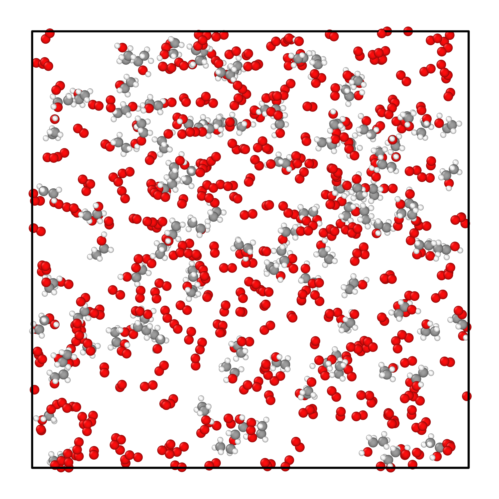
Initial system configuration
2. Simulation
When system prepared, we will use GPUMD to perform a 200 ps molecular dynamics simulation. According to the
adiabatic combustion temperature of ethanol, which is 2082 ℃, ~2350 K, we will set the simulation
temperature as 2350 K. And the ensemble is NVT, using langevin thermostat.
The GPUMD running parameter file run.in as below:
            potential    nep.txt
            velocity     2350
            time_step    0.2

            ensemble     nvt_lan 2350 2350 100
            dump_thermo   10
            dump_exyz     500
            run           1000000
We will use the newest Neuroevolution Potential (NEP) parameter set NEP-89 for simulation. Before simulation,
the working directory contains files below:
run.in nep.txt model.xyz
Use command
gpumd directly to invoke an automatic GPUMD task in current directory.
The simulation cost 10~20 minutes on GTX 4090D machine, after simulation terminated, the system structure
looks like below:
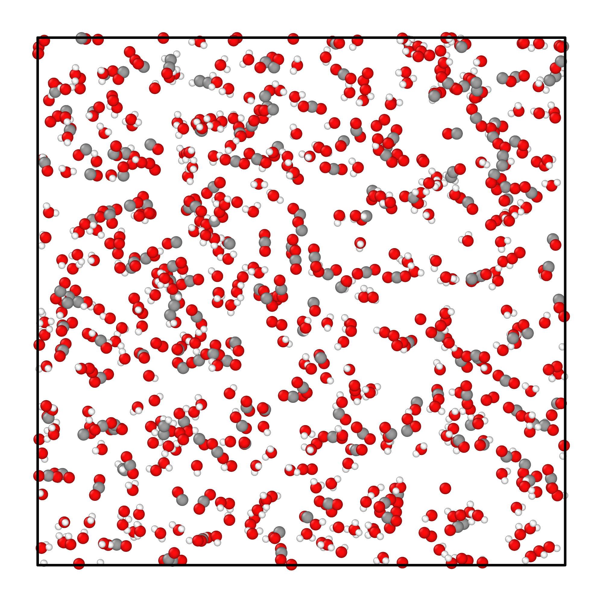
System configuration after simulation.
3. ReaxTools Analysis
After simulation completion, GPUMD outputs a standard trajectory file (dump.xyz) in the current
directory. This file is compatible with ReaxTools (File format reference).
Analysis steps:
- Load the file on the main page
- Click "Run" (typically completes within 1 minute)
- View clearly presented results on the website
Configuration tip: For this case, we use -r 1 to apply stricter bond cutoff
criteria for molecular identification. For advanced customization, see Input
options reference.
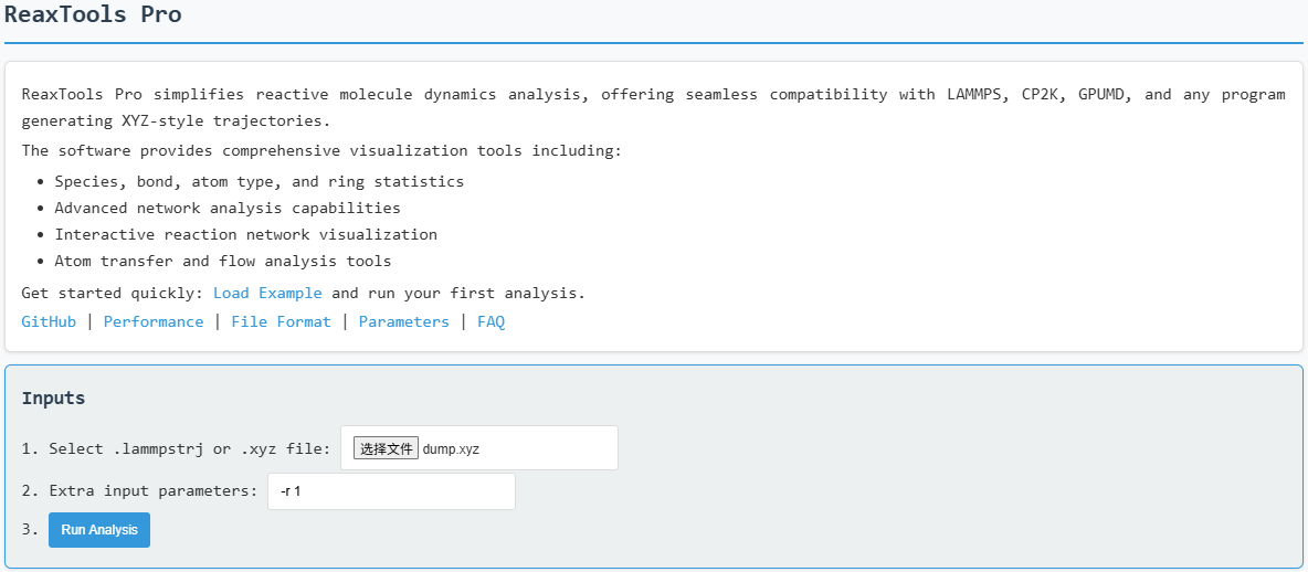
Loading input file with analysis options
Key results from the simulation are presented below:
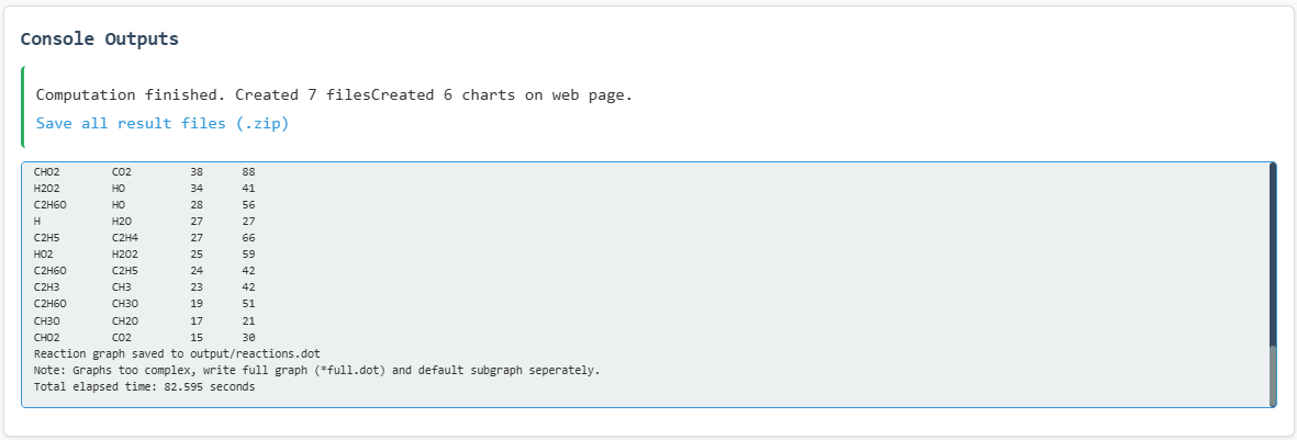
Program execution log output
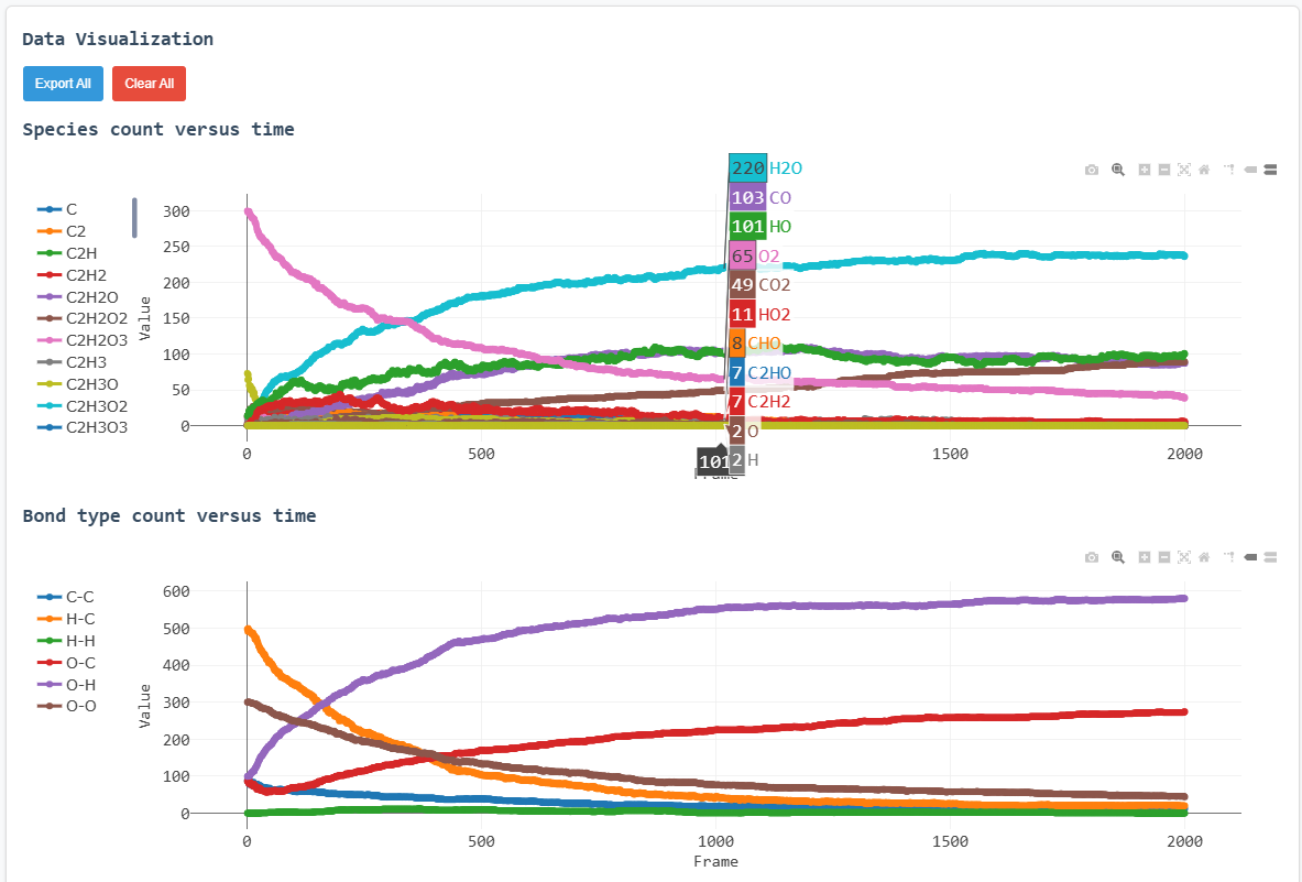
Species count versus time (complete view)
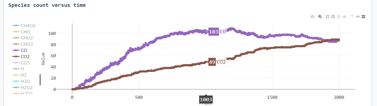
Species count versus time (focused view)
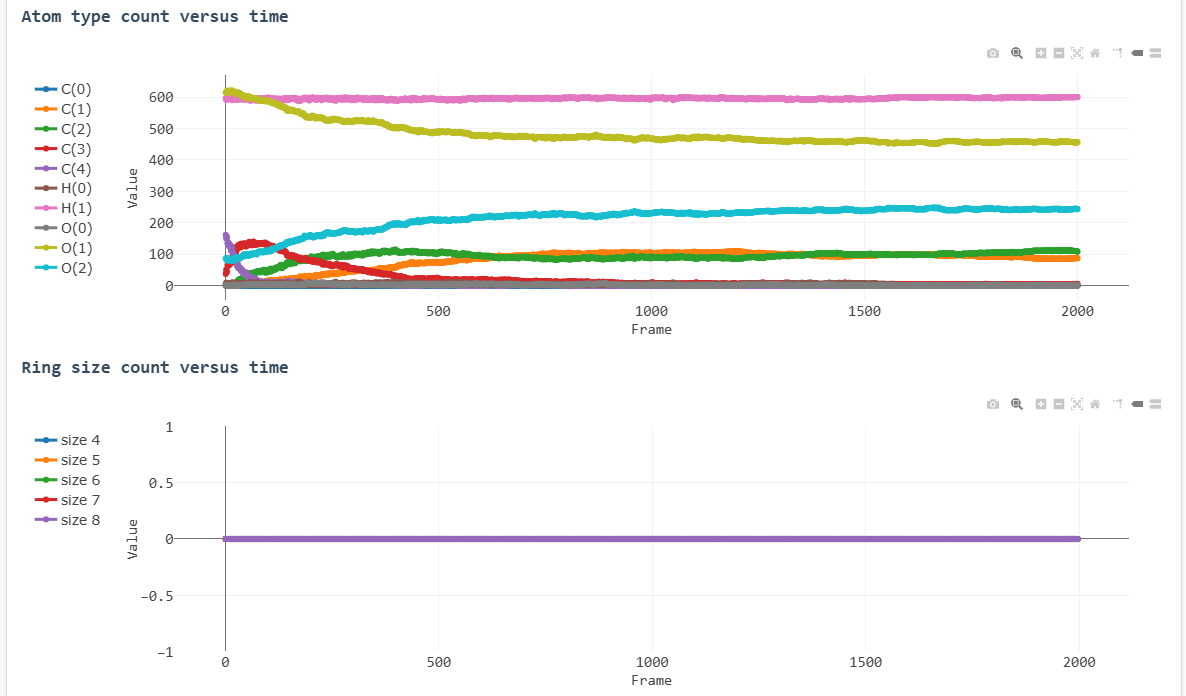
Atom type count versus time
Atom type legend:
- C(3): sp² hybridized carbons
- C(2): sp hybridized carbons
- C(1): Primarily CO, occasionally CH/CC fragments
- O(0): Isolated oxygen atoms
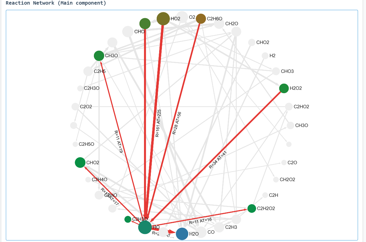
OH fragment reaction network (radical/anion focused)
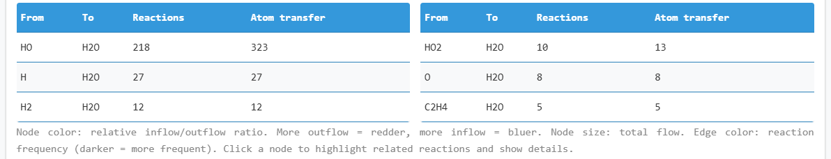
OH-related reaction pathways table
The network visualization displays the main reaction components. Hover over elements to view associated
reactions and molecules.
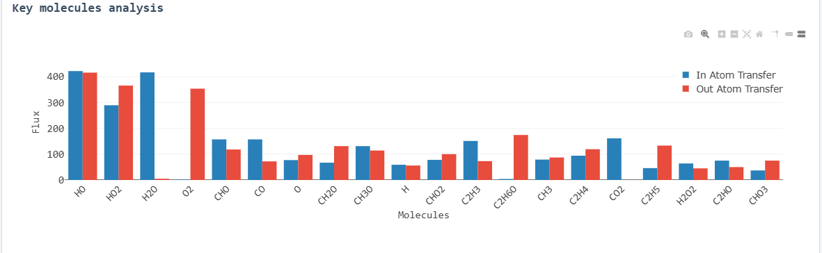
Key molecule reaction fluxes
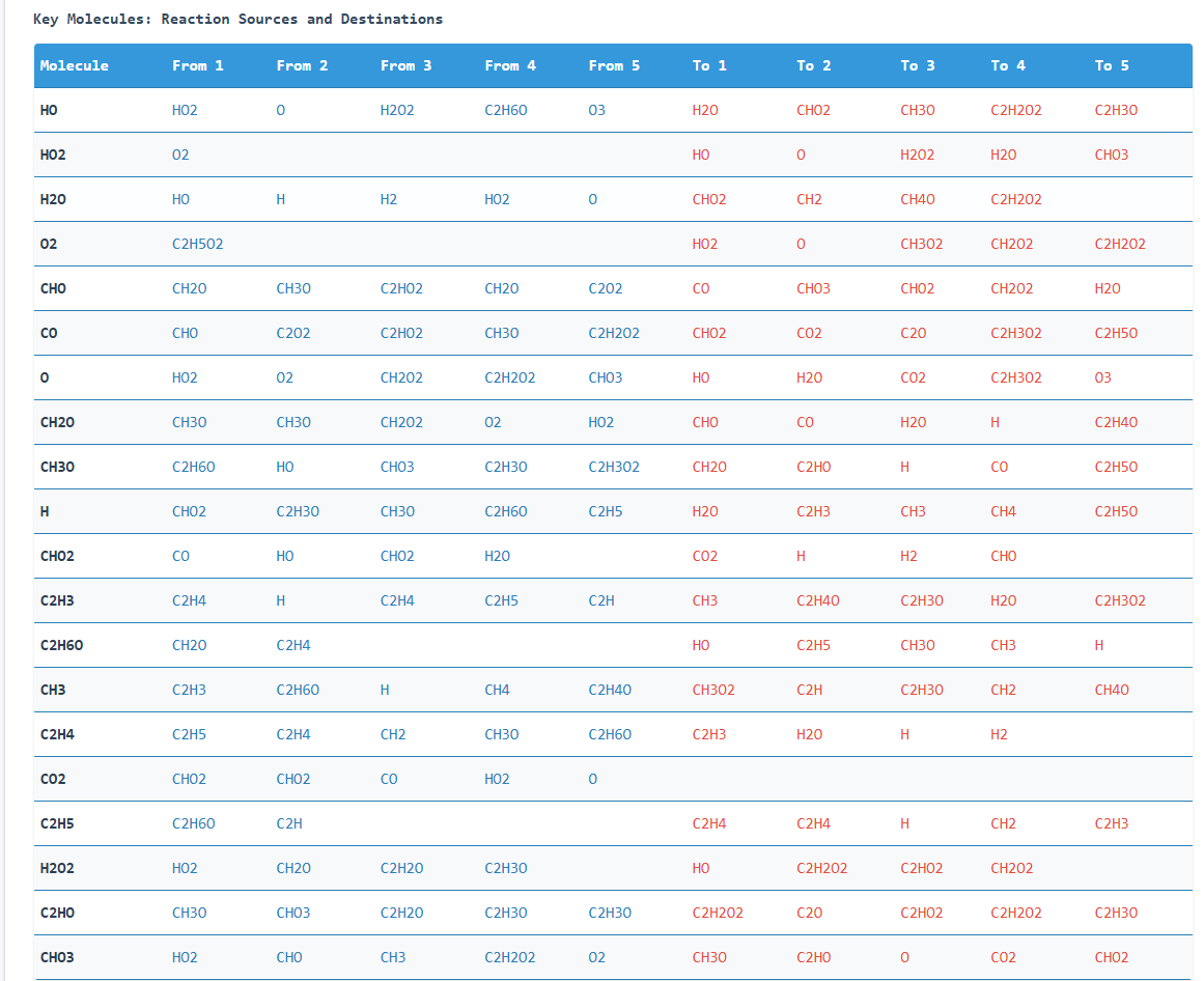
Key molecule reaction partners table
Key molecules (those with high reaction frequency) are identified through their flux values. The
visualizations and tables help analyze:
- Which molecules react most frequently
- Their reaction rates
- Their source molecules and reaction products